• Skip to primary navigation
  • Skip to main content
  • Skip to footer
Bluetab

Bluetab

an IBM Company

  • SOLUTIONS
    • DATA STRATEGY
    • Data Readiness
    • Data Products AI
  • Assets
    • TRUEDAT
    • FASTCAPTURE
    • Spark Tune
  • About Us
  • Our Offices
    • Spain
    • Mexico
    • Peru
    • Colombia
  • talent
    • Spain
    • TALENT HUB BARCELONA
    • TALENT HUB BIZKAIA
    • TALENT HUB ALICANTE
    • TALENT HUB MALAGA
  • Blog
  • EN
    • ES

Tech

MDM as a Competitive Advantage in Organizations

June 18, 2024 by Bluetab

MDM as a Competitive Advantage in Organizations

Maryury García

Cloud | Data & Analytics

Just like natural resources, data acts as the driving fuel for innovation, decision-making, and value creation across various sectors. From large tech companies to small startups, digital transformation is empowering data to become the foundation that generates knowledge, optimizes efficiency, and offers personalized experiences to users.

Master Data Management (MDM) plays an essential role in providing a solid structure to ensure the integrity, quality, and consistency of data throughout the organization.

Despite this discipline existing since the mid-90s, some organizations have not fully adopted MDM. This could be due to various factors such as a lack of understanding of its benefits, cost, complexity, and/or maintenance.

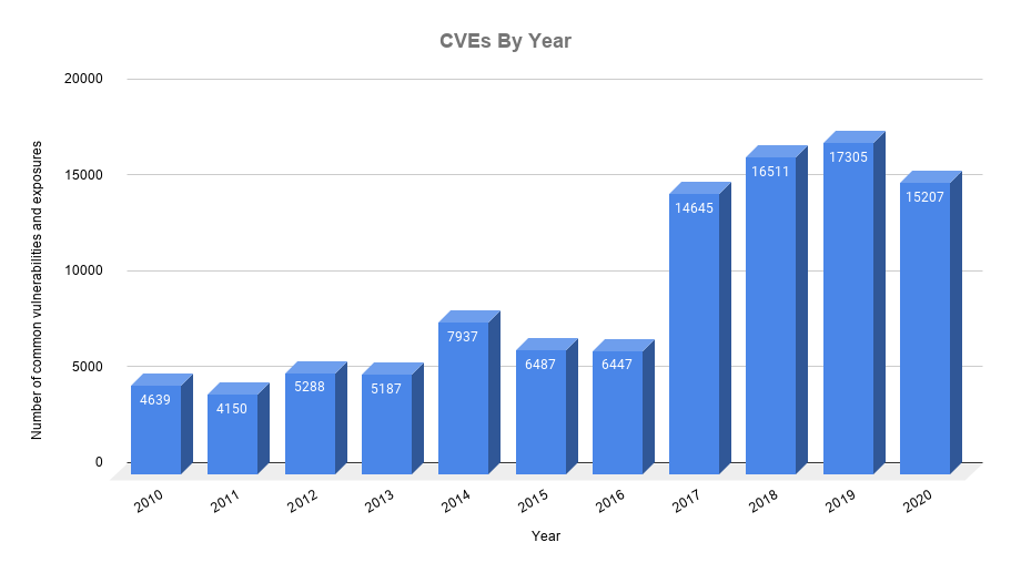
According to a Gartner survey, the global MDM market was valued at $14.6 billion in 2022 and is expected to reach $24 billion by 2028, with a compound annual growth rate (CAGR) of 8.2%.

Figura 01: CAGR en el mercado global MDM

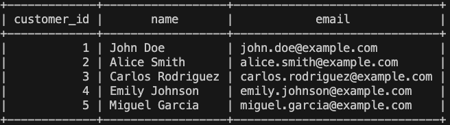
Before diving into the world of MDM, it is important to understand some relevant concepts. To manage master data, the first question we ask is: What is master data? Master data constitutes the set of shared, essential, and critical data for business execution. It has a lifecycle (validity period) and contains key information for the organization’s operation, such as customer data, product information, account numbers, and more.

Once defined, it is important to understand their characteristics, as master data is unique, persistent, and integral, with broad coverage, among other qualities. This is vital to ensure consistency and quality.

Therefore, it is essential to have an approach that considers both organizational aspects (identification of data owners, impacted users, matrices, etc.) as well as processes (related to policies, workflows, procedures, and mappings). Hence, our proposal at Bluetab on this approach is summarized in each of these dimensions.

Figura 02: Caso de Uso: Enfoque Datos Maestros

Another aspect to consider from our experience with master data, which is key to starting an organizational implementation, is understanding its “lifecycle.” This includes:

  • The business areas inputting the master data (referring to the areas that will consume the information).
  • The processes associated with the master data (that create, block, report, update the master data attributes—in other words, the treatment that the master data will undergo).
  • The areas outputting the master data (referring to the areas that ultimately maintain the master data).
  • All of this is intertwined with the data owners and supported by associated policies, procedures, and documentation.
Figura 03: Caso de Uso: Matriz del ciclo de vida del Dato Maestro

Master Data Management (MDM) is a “discipline,” and why? Because it brings together a set of knowledge, policies, practices, processes, and technologies (referred to as a technological tool to collect, store, manage, and analyze master data). This allows us to conclude that it is much more than just a tool.

Below, we provide some examples that will help to better understand the contribution of proper master data management in various sectors:

  • Retail Sector: Retail companies, for example, a bakery, would use MDM to manage master data for product catalogs, customers, suppliers, employees, recipes, inventory, and locations. This creates a detailed customer profile to ensure a consistent and personalized shopping experience across all sales channels.
  • Financial Sector: Financial institutions could manage customer data, accounts, financial products, pricing, availability, historical transactions, and credit information. This helps improve the accuracy and security of financial transactions and operations, as well as verify customer identities before opening an account.
  • Healthcare Sector: In healthcare, the most important data is used to manage patient data, procedure data, diagnostic data, imaging data, medical facilities, and medications, ensuring the integrity and privacy of confidential information. For example, a hospital can use MDM to generate an EMR (Electronic Medical Record) for each patient.
  • Telecommunications Sector: In telecommunications, companies use MDM to manage master data for their devices, services, suppliers, customers, and billing.

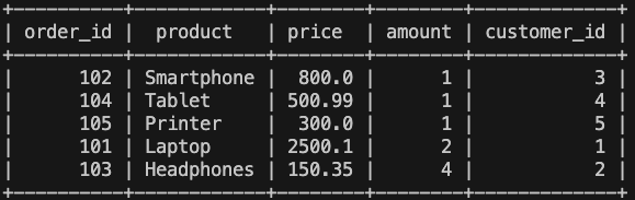
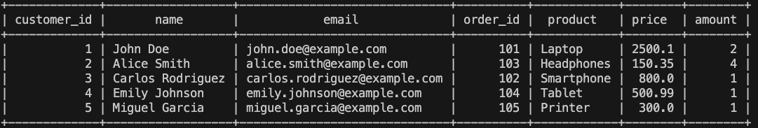
In Master Data Management, the following fundamental operations are performed: data cleaning, which removes duplicates; data enrichment, which ensures complete records; and the establishment of a single source of truth. The time it may take depends on the state of the organization’s records and its business objectives. Below, we can visualize the tasks that are carried out:

Figura 04: Tareas claves MDM

Now that we have a clearer concept, it’s important to keep in mind that the strategy for managing master data is to keep it organized: up-to-date, accurate, non-redundant, consistent, and integral.

What benefits does implementing an MDM provide?

  • Data Quality and Consistency: Improves the quality of master data by eliminating duplicates and correcting errors, ensuring the integrity of information throughout the organization.
  • Efficiency and Resource Savings: Saves time and resources by automating tasks of data cleaning, enrichment, and updating, freeing up staff for more strategic tasks.
  • Informed Decision-Making: Allows the identification of patterns and trends from reliable data, driving strategic and timely decision-making.
  • Enhanced Customer Experience: Improves the customer experience by providing a 360-degree view of the customer, enabling more personalized and relevant interactions.
  • At Bluetab, we have helped clients from various industries with their master data strategy, from the definition, analysis, and design of the architecture to the implementation of an integrated solution. From this experience, we share these 5 steps to help you start managing master data:

List Your Objectives and Define a Scope

First, identify which data entities are of commercial priority within the organization. Once identified, evaluate the number of sources, definitions, exceptions, and volumes that the entities have.

Define the Data You Will Use

Which part of the data is important for decision-making? It could simply be all or several fields of the record to fill in, such as name, address, and phone number. Get support from governance personnel for the definition.

Establish Processes and Owners

Who will be responsible for having the rights to modify or create the data? For what and how will this data be used to reinforce or enhance the business? Once these questions are formulated, it is important to have a process for how the information will be handled from the master data registration to its final sharing (users or applications).

Seek Scalability

Once you have defined the processes, try to ensure they can be integrated with future changes. Take the time to define your processes and avoid making drastic changes in the future.

Find the Right Data Architecture, Don’t Take Shortcuts

Once the previous steps are defined and generated, it’s time to approach your Big Data & Analytics strategic partner to ensure these definitions are compatible within the system or databases that house your company’s information.

Figura 05: Primeros Pasos MDM

Final Considerations

Based on our experience, we suggest considering the following aspects when assessing/defining the process for each domain in master data management, subject to the project scope:

  • Management of Routes:
    • Consider how the owner of the creation of master data registers it (automatically and eliminating manual data entry from any other application) and how any current process of an area/person centralizes the information from other areas involved in the master data manually (emails, calls, Excel sheets, etc.). This should be automated in a workflow.
  • Alerts & Notifications:
    • It is recommended to establish deadlines for the completeness of the data for each area and the responsible party updating a master data.
    • The time required to complete each data entry should be agreed upon among all involved areas, and alerts should be configured to communicate the updated master data.
  • Blocking and Discontinuation Processes:
    • A viable alternative is to make these changes operationally and then communicate them to the MDM through replication.
  • Integration:
    • Evaluate the possibility of integrating with third parties to automate the registration process for clients, suppliers, etc., and avoid manual entry: RENIEC, SUNAT, Google (coordinates X, Y, Z), or other agents, evaluating suitability for the business.
  • Incorporation of Third Parties:
    • Consider the incorporation of clients and suppliers at the start of the master data creation flows and at the points of updating.
Figura 06: Aspectos a considerar MDM

In summary, master data is the most important common data for an organization and serves as the foundation for many day-to-day processes at the enterprise level. Master data management helps ensure that data is up-to-date, accurate, non-redundant, consistent, integral, and properly shared, providing tangible benefits in data quality, operational efficiency, informed decision-making, and customer experience. This contributes to the success and competitiveness of the organization in an increasingly data-driven digital environment.

If you found this article interesting, we appreciate you sharing it. At Bluetab, we look forward to hearing about the challenges and needs you have in your organization regarding master and reference data.

Maryury García

Cloud | Data & Analytics

Do you want to learn more about what we offer and see other success stories?
DISCOVER BLUETAB

SOLUCIONES, SOMOS EXPERTOS

DATA STRATEGY
DATA FABRIC
AUGMENTED ANALYTICS

Te puede interesar

Cómo depurar una Lambda de AWS en local

October 8, 2020
LEER MÁS

El futuro del Cloud y GenIA en el Next ’23

September 19, 2023
LEER MÁS

Serverless Microservices

October 14, 2021
LEER MÁS

Mi experiencia en el mundo de Big Data – Parte I

October 14, 2021
LEER MÁS

Desplegando una plataforma CI/CD escalable con Jenkins y Kubernetes

September 22, 2021
LEER MÁS

How much is your customer worth?

October 1, 2020
LEER MÁS

Filed Under: Blog, Tech

Boost Your Business with GenAI and GCP: Simple and for Everyone

March 27, 2024 by Bluetab

Alfonso Zamora
Cloud Engineer

Introduction

The main goal of this article is to present a solution for data analysis and engineering from a business perspective, without requiring specialized technical knowledge.

Companies have a large number of data engineering processes to extract the most value from their business, and sometimes, very complex solutions for the required use case. From here, we propose to simplify the operation so that a business user, who previously could not carry out the development and implementation of the technical part, will now be self-sufficient, and will be able to implement their own technical solutions with natural language.

To fulfill our goal, we will make use of various services from the Google Cloud platform to create both the necessary infrastructure and the different technological components to extract all the value from business information.

Before we begin

Before we begin with the development of the article, let’s explain some basic concepts about the services and different frameworks we will use for implementation:

  1. Cloud Storage[1]: It is a cloud storage service provided by Google Cloud Platform (GCP) that allows users to securely and scalably store and retrieve data.
  2. BigQuery[2]: It is a fully managed data analytics service that allows you to run SQL queries on massive datasets in GCP. It is especially effective for large-scale data analysis.
  3. Terraform[3]: It is an infrastructure as code (IaC) tool developed by HashiCorp. It allows users to describe and manage infrastructure using configuration files in the HashiCorp Configuration Language (HCL). With Terraform, you can define resources and providers declaratively, making it easier to create and manage infrastructure on platforms like AWS, Azure, and Google Cloud.
  4. PySpark[4]: It is a Python interface for Apache Spark, an open-source distributed processing framework. PySpark makes it easy to develop parallel and distributed data analysis applications using the power of Spark.
  5. Dataproc[5]: It is a cluster management service for Apache Spark and Hadoop on GCP that enables efficient execution of large-scale data analysis and processing tasks. Dataproc supports running PySpark code, making it easy to perform distributed operations on large datasets in the Google Cloud infrastructure.

What is an LLM?

An LLM (Large Language Model) is a type of artificial intelligence (AI) algorithm that utilizes deep learning techniques and massive datasets to comprehend, summarize, generate, and predict new content. An example of an LLM could be ChatGPT, which makes use of the GPT model developed by OpenAI.

In our case, we will be using the Codey model (code-bison), which is a model implemented by Google that is optimized for generating code as it has been trained specifically for this specialization, which is part of the VertexAI stack.

However, it’s not only important which model we are going to use, but also how we are going to use it. By this, I mean it’s necessary to understand the input parameters that directly affect the responses our model will provide, among which we can highlight the following:

  • Temperature: This parameter controls the randomness in the model’s predictions. A low temperature, such as 0.1, generates more deterministic and focused results, while a high temperature, such as 0.8, introduces more variability and creativity in the model’s responses.
  • Prefix (Prompt): The prompt is the input text provided to the model to initiate text generation. The choice of prompt is crucial as it guides the model on the specific task expected to be performed. The formulation of the prompt can influence the quality and relevance of the model’s responses, although the length should be considered to meet the maximum number of input tokens, which is 6144.
  • Output Tokens (max_output_tokens): This parameter limits the maximum number of tokens that will be generated in the output. Controlling this value is useful for avoiding excessively long responses or for adjusting the output length according to the specific requirements of the application.
  • Candidate Count: This parameter controls the number of candidate responses the model generates before selecting the best option. A higher value can be useful for exploring various potential responses, but it will also increase computational cost.

Development of the prompt

Once we have defined the parameters and understand well what each of them is for, and we comprehend what a prompt is, let’s focus on how to use it and implement one that can adapt to our needs.

As mentioned earlier, the goal is to generate both PySpark code and Terraform in order to perform infrastructure creation and data processing tasks. Since these are completely different tasks, as a first important decision for our prompt, we have chosen to divide it into two specific parts so that each prompt is trained with examples to generate one language or the other.

For each prompt, an introduction is made to specify what the objective will be and what requests will be made, followed by a series of examples in which input in natural language is given simulating a request, and then the desired output is also given to assign the text to the specific code. The goal is to generate a structured prompt that can be efficiently processed by the model so that in the following cases, it can associate the available examples with appropriate responses.

Let’s put these small tips into practice to see one of the entries to the Terraform prompt:

input: I need to read a file named `myfile.csv` inside the folder `data/input` in a bucket called `application-data-input`, and I need to create a new dataset and table in BigQuery called `tst_tf_ai`. The process has to read the file, remove the first three characters of the name, and write the result in BigQuery. The schema of the table will be ‘name’ of String type and ‘surname’ of String type. The infrastructure has to be deployed in the project `project-cloud-223` in GCP, and region `europe-southwest1`.
output: “`hcl
terraform {
 required_version = “>= 0.15”
 required_providers {
  google = “~> 5.0”
 }
}

resource “google_storage_bucket” “temporary_files” { 
 project       = “project-cloud-223” 
 name          = “temporary-files-dataproc” 
 location      = “europe-southwest1” 
 force_destroy = true 
} 

resource “google_storage_bucket” “bucket1” { 
 project       = “project-cloud-223” 
 name          = “application-data-input” 
 location      = “europe-southwest1” 
 force_destroy = true 
} 

resource “google_storage_bucket_object” “folder1” {
 name    = “data/input/”
 bucket  = google_storage_bucket.bucket1.name
 content = ” “
}

resource “google_bigquery_dataset” “dataset” { 
 project       = “project-cloud-223” 
 dataset_id    = “tst_tf_ai” 
 friendly_name = “tst_tf_ai” 
 description   = “Description” 
 location      = “europe-southwest1” 
} 

resource “google_bigquery_table” “table” { 
 project              = “project-cloud-223” 
 dataset_id           = google_bigquery_dataset.dataset.dataset_id 
 deletion_protection  = false
 table_id             = “tst_tf_ai” 
 schema               = <<EOF
[ 
 { 
  “name”: “name”, 
  “type”: “STRING”, 
  “mode”: “NULLABLE”, 
  “description”: “The name” 
 }, 
 { 
  “name”: “surname”, 
  “type”: “STRING”, 
  “mode”: “NULLABLE”, 
  “description”: “The surname” 
 }
] 
EOF 
} 
“`

Author Name

It’s important to implement examples as closely as possible to your use case so that the responses are more accurate, and also to have plenty of examples with a variety of requests to make it smarter when returning responses. One of the practices to make the prompt implementation more interactive could be to try different requests, and if it’s unable to do what’s been asked, the instructions should be modified.

As we have observed, developing the prompt does require technical knowledge to translate requests into code, so this task should be tackled by a technical person to subsequently empower the business user. In other words, we need a technical person to generate the initial knowledge base so that business users can then make use of these types of tools.

It has also been noticed that generating code in Terraform is more complex than generating code in PySpark, so more input examples were required in creating the Terraform prompt to tailor it to our use case. For example, we have applied in the examples that in Terraform it always creates a temporary bucket (temporary-files-dataproc) so that it can be used by Dataproc.

Practical Cases

Three examples have been carried out with different requests, requiring more or less infrastructure and transformations to see if our prompt is robust enough.

In the file ai_gen.py, we see the necessary code to make the requests and the three examples, in which it is worth highlighting the configuration chosen for the model parameters:

  • It has been decided to set the value of candidate_count to 1 so that it has no more than one valid final response to return. Additionally, as mentioned, increasing this number also entails increased costs.
  • The max_output_tokens has been set to 2048, which is the highest number of tokens for this model, as if it needs to generate a response with various transformations, it won’t fail due to this limitation.
  • The temperature has been varied between the Terraform and PySpark code. For Terraform, we have opted for 0 so that it always gives the response that is considered closest to our prompt, ensuring it doesn’t generate more than strictly necessary for our objective. In contrast, for PySpark, we have opted for 0.2, which is a low temperature to prevent excessive creativity, yet still allowing it to provide diverse responses with each call, enabling performance testing among them.

We are going to carry out an example of a request that is available in the following GitHub repository, where it is detailed step by step in the README to be able to execute it yourself. The request is as follows:

In the realm of ‘customer_table,’ my objective is the seamless integration of pivotal fields such as ‘customer_id’, ‘name’, and ’email’. These components promise to furnish crucial insights into the essence of our valued customer base.

Conversely, when delving into the nuances of ‘sales_table,’ the envisioned tapestry includes essential elements like ‘order_id’ ‘product’ ‘price’, ‘amount’ and ‘customer_id’. Theseattributes, meticulously curated, will play a pivotal role in the nuanced exploration and analysis of sales-related data.

The ‘bigtable_info’ table will have all the fields resulting from the union of the two tables, ‘customer_table’ and ‘sales_table.’ Here, the outcome of joining the two tables by the ‘customer_id’ numeric field will be stored.

Furthermore, as part of our meticulous data collection strategy, I plan to inaugurate a dedicated Google Cloud Storage bucket christened ‘sales-etl-bucket.’ This repository is strategically designed to serve as a robust container for collating data, particularly hailing from CSV files. This endeavor is set to enhance the efficiency and organizational prowess of our data management processes.

To enhance the structure, two distinct subfolders, ‘input/sales’ and ‘input/customers’ have been ingeniously incorporated within the ‘sales-etl-bucket,’ ensuring a refined organization of the incoming data streams.

You will need to read the CSV files within the ‘input/sales’ folder to write the data into the ‘sales_table’. Additionally, you should perform the same operation with the files from the ‘input/customers’ folder to write the data into the ‘customer_table’. Finally, you are required to perform a join between the sales and customers information based on the ‘customer_id’ number field and write the merged information into the ‘bigtable_info’.

Author Name

We execute and will analyze the outputs generated in the folders generated/customers/python/etl.py and generated/terraform/main.tf.

terraform {
 required_version = ">= 0.15"
 required_providers {
   google = "~> 5.0"
 }
}


resource "google_storage_bucket" "temporary_files" {
 project       = "my-cloud-project"
 name          = "temporary-files-dataproc"
 location      = "europe-southwest1"
 force_destroy = true
}


resource "google_storage_bucket" "sales_etl_bucket" {
 project       = "my-cloud-project"
 name          = "sales-etl-bucket"
 location      = "europe-southwest1"
 force_destroy = true
}


resource "google_storage_bucket_object" "sales_folder" {
 name    = "input/sales/"
 bucket  = google_storage_bucket.sales_etl_bucket.name
 content = " "
}


resource "google_storage_bucket_object" "customers_folder" {
 name    = "input/customers/"
 bucket  = google_storage_bucket.sales_etl_bucket.name
 content = " "
}


resource "google_bigquery_dataset" "raw_sales_data" {
 project       = "my-cloud-project"
 dataset_id    = "raw_sales_data"
 friendly_name = "Raw Sales Data"
 description   = "This dataset contains the raw sales data."
 location      = "europe-southwest1"
}


resource "google_bigquery_table" "customer_table" {
 project              = "my-cloud-project"
 dataset_id           = google_bigquery_dataset.raw_sales_data.dataset_id
 deletion_protection  = false
 table_id             = "customer_table"
 schema               = <<EOF
[
 {
   "name": "customer_id",
   "type": "INT64",
   "mode": "REQUIRED",
   "description": "The customer ID."
 },
 {
   "name": "name",
   "type": "STRING",
   "mode": "NULLABLE",
   "description": "The customer's name."
 },
 {
   "name": "email",
   "type": "STRING",
   "mode": "NULLABLE",
   "description": "The customer's email address."
 }
]
EOF
}


resource "google_bigquery_table" "sales_table" {
 project              = "my-cloud-project"
 dataset_id           = google_bigquery_dataset.raw_sales_data.dataset_id
 deletion_protection  = false
 table_id             = "sales_table"
 schema               = <<EOF
[
 {
   "name": "order_id",
   "type": "INT64",
   "mode": "REQUIRED",
   "description": "The order ID."
 },
 {
   "name": "product",
   "type": "STRING",
   "mode": "NULLABLE",
   "description": "The product name."
 },
 {
   "name": "price",
   "type": "FLOAT64",
   "mode": "NULLABLE",
   "description": "The product price."
 },
 {
   "name": "amount",
   "type": "INT64",
   "mode": "NULLABLE",
   "description": "The product amount."
 },
 {
   "name": "customer_id",
   "type": "INT64",
   "mode": "REQUIRED",
   "description": "The customer ID."
 }
]
EOF
}


resource "google_bigquery_dataset" "master_sales_data" {
 project       = "my-cloud-project"
 dataset_id    = "master_sales_data"
 friendly_name = "Master Sales Data"
 description   = "This dataset contains the master sales data."
 location      = "europe-southwest1"
}


resource "google_bigquery_table" "bigtable_info" {
 project              = "my-cloud-project"
 dataset_id           = google_bigquery_dataset.master_sales_data.dataset_id
 deletion_protection  = false
 table_id             = "bigtable_info"
 schema               = <<EOF
[
 {
   "name": "customer_id",
   "type": "INT64",
   "mode": "REQUIRED",
   "description": "The customer ID."
 },
 {
   "name": "name",
   "type": "STRING",
   "mode": "NULLABLE",
   "description": "The customer's name."
 },
 {
   "name": "email",
   "type": "STRING",
   "mode": "NULLABLE",
   "description": "The customer's email address."
 },
 {
   "name": "order_id",
   "type": "INT64",
   "mode": "REQUIRED",
   "description": "The order ID."
 },
 {
   "name": "product",
   "type": "STRING",
   "mode": "NULLABLE",
   "description": "The product name."
 },
 {
   "name": "price",
   "type": "FLOAT64",
   "mode": "NULLABLE",
   "description": "The product price."
 },
 {
   "name": "amount",
   "type": "INT64",
   "mode": "NULLABLE",
   "description": "The product amount."
 }
]
EOF
}


We see that it will add a bucket with two folders to upload the data to the corresponding folder depending on whether it is sales or customer data. It has also created two datasets, one for the raw layer to have the data as it came from the source with the tables of customers and sales, and the second dataset for the final table that will store the result of joining the information from both tables.

Let’s review the PySpark code:

from pyspark.sql import SparkSession
from pyspark.sql import functions as F


# Configure Spark session
spark = SparkSession.builder.appName("SalesETL").getOrCreate()


# Define file paths
sales_path = "gs://sales-etl-bucket/input/sales/*.csv"
customers_path = "gs://sales-etl-bucket/input/customers/*.csv"


# Read CSV files into DataFrames
sales_df = spark.read.csv(sales_path, header=True, inferSchema=True)
customers_df = spark.read.csv(customers_path, header=True, inferSchema=True)


# Write tables to BigQuery
sales_df.write.format("bigquery") \
   .option("temporaryGcsBucket", "temporary-files-dataproc") \
   .option("table",  "raw_sales_data.sales_table") \
   .mode("overwrite") \
   .save()
customers_df.write.format("bigquery") \
   .option("temporaryGcsBucket", "temporary-files-dataproc") \
   .option("table",  "raw_sales_data.customer_table") \
   .mode("overwrite") \
   .save()


# Join sales and customers tables
bigtable_info_df = sales_df.join(customers_df, on="customer_id", how="inner")


# Write joined table to BigQuery
bigtable_info_df.write.format("bigquery") \
   .option("temporaryGcsBucket", "temporary-files-dataproc") \
   .option("table",  "master_sales_data.bigtable_info") \
   .mode("overwrite") \
   .save()


# Stop the Spark session
spark.stop()

It can be observed that the generated code reads from each of the folders and inserts each data into its corresponding table.

Para poder asegurarnos de que el ejemplo está bien realizado, podemos seguir los pasos del README en el repositorio GitHub[8] para aplicar los cambios en el código terraform, subir los ficheros de ejemplo que tenemos en la carpeta example_data y a ejecutar un Batch en Dataproc. 

Finally, we check if the information stored in BigQuery is correct:

  • Table customer:
  • Tabla sales:
  • Final table:

This way, we have managed to have a fully operational functional process through natural language. There is another example that can be executed, although I also encourage creating more examples, or even improving the prompt, to incorporate more complex examples and also adapt it to your use case.

Conclusions and Recommendations

As the examples are very specific to particular technologies, any change in the prompt in any example can affect the results, or also modifying any word in the input request. This means that the prompt is not robust enough to assimilate different expressions without affecting the generated code. To have a productive prompt and system, more training and different variety of solutions, requests, expressions, etc., are needed. With all this, we will finally be able to have a first version to present to our business user so that they can be autonomous.

Specifying the maximum possible detail to an LLM is crucial for obtaining precise and contextual results. Here are several tips to keep in mind to achieve appropriate results:

  • Clarity and Conciseness:
    • Be clear and concise in your prompt, avoiding long and complicated sentences.
    • Clearly define the problem or task you want the model to address.
  • Specificity:
    • Provide specific details about what you are looking for. The more precise you are, the better results you will get.
  • Variability and Diversity:
    • Consider including different types of examples or cases to assess the model’s ability to handle variability.
  • Iterative Feedback:
    • If possible, iterate on your prompt based on the results obtained and the model’s feedback.
  • Testing and Adjustment:
    • Before using the prompt extensively, test it with examples and adjust as needed to achieve desired results.

Future Perspectives

In the field of LLMs, future lines of development focus on improving the efficiency and accessibility of language model implementation. Here are some key improvements that could significantly enhance user experience and system effectiveness:

1. Use of different LLM models:

The inclusion of a feature that allows users to compare the results generated by different models would be essential. This feature would provide users with valuable information about the relative performance of the available models, helping them select the most suitable model for their specific needs in terms of accuracy, speed, and required resources.

2. User feedback capability:

Implementing a feedback system that allows users to rate and provide feedback on the generated responses could be useful for continuously improving the model’s quality. This information could be used to adjust and refine the model over time, adapting to users’ changing preferences and needs.

3. RAG (Retrieval-augmented generation)

RAG (Retrieval-augmented generation) is an approach that combines text generation and information retrieval to enhance the responses of language models. It involves using retrieval mechanisms to obtain relevant information from a database or textual corpus, which is then integrated into the text generation process to improve the quality and coherence of the generated responses.

Links of Interest

Cloud Storage[1]: https://cloud.google.com/storage/docs

BigQuery[2]: https://cloud.google.com/bigquery/docs

Terraform[3]: https://developer.hashicorp.com/terraform/docs

PySpark[4]: https://spark.apache.org/docs/latest/api/python/index.html

Dataproc[5]: https://cloud.google.com/dataproc/docs

Codey[6]: https://cloud.google.com/vertex-ai/generative-ai/docs/model-reference/code-generation

VertexAI[7]: https://cloud.google.com/vertex-ai/docs

GitHub[8]: https://github.com/alfonsozamorac/etl-genai

Table Of Contents
  1. Introduction
  2. Before we begin
  3. What is an LLM?
  4. Development of the prompt
  5. Practical Cases

Filed Under: Blog, Practices, Tech

Container vulnerability scanning with Trivy

March 22, 2024 by Bluetab

Container vulnerability scanning
with Trivy

Ángel Maroco

AWS Cloud Architect

Within the framework of security in container, the build phase is of vital importance as we need to select the base image on which applications will run. Not having automatic mechanisms for vulnerability scanning can lead to production environments with insecure applications with the risks that involves.

In this article we will cover vulnerability scanning using Aqua Security’s Trivy solution, but before we begin, we need to explain what the basis is for these types of solutions for identifying vulnerabilities in Docker images.

Introduction to CVE (Common Vulnerabilities and Exposures)

CVE is a list of information maintained by MITRE Corporation which is aimed at centralising the records of known security vulnerabilities, where each reference has a CVE-ID number, description of the vulnerability, which versions of the software are affected, possible fix for the flaw (if any) or how to configure to mitigate the vulnerability and references to publications or posts in forums or blogs where the vulnerability has been made public or its exploitation is demonstrated.

The CVE-ID provides a standard naming convention for uniquely identifying a vulnerability. They are classified into 5 typologies, which we will look at in the Interpreting the analysis section. These types are assigned based on different metrics (if you are curious, see CVSS Calculator v3).

CVE has become the standard for vulnerability recording, so it is used by the great majority of technology companies and individuals.

There are various channels for keeping informed of all the news related to vulnerabilities: official blog, Twitter, cvelist on GitHub and LinkedIn.

If you want more detailed information about a vulnerability, you can also consult the NIST website, specifically the NVD (National Vulnerability Database).

We invite you to search for one of the following critical vulnerabilities. It is quite possible that they have affected you directly or indirectly. We should forewarn you that they have been among the most discussed data-src=

  • CVE-2017-5753
  • CVE-2017-5754

If you detect a vulnerability, we encourage you to register it using the form below.

Aqua Security – Trivy

Trivy is an open source tool focused on detecting vulnerabilities in OS-level packages and dependency files for various languages:

  • OS packages: (Alpine, Red Hat Universal Base Image, Red Hat Enterprise Linux, CentOS, Oracle Linux, Debian, Ubuntu, Amazon Linux, openSUSE Leap, SUSE Enterprise Linux, Photon OS and Distroless)

  • Application dependencies: (Bundler, Composer, Pipenv, Poetry, npm, yarn and Cargo)

Aqua Security, a company specialising in development of security solutions, acquired Trivy in 2019. Together with a substantial number of collaborators, they are responsible for developing and maintaining it.

Installation

Trivy has installers for most Linux and MacOS systems. For our tests, we will use the generic installer:

curl -sfL https://raw.githubusercontent.com/aquasecurity/trivy/master/contrib/install.sh | sudo sh -s -- -b /usr/local/bin 

If we do not want to persist the binary on our system, we have a Docker image:

docker run --rm -v /var/run/docker.sock:/var/run/docker.sock -v /tmp/trivycache:/root/.cache/ aquasec/trivy python:3.4-alpine 

Basic operations

  • Local images

Trivy has installers for most Linux and MacOS systems. For our tests, we will use the generic installer:

#!/bin/bash
docker build -t cloud-practice/alpine:latest -<<EOF
FROM alpine:latest
RUN echo "hello world"
EOF

trivy image cloud-practice/alpine:latest 
  • Remote images
#!/bin/bash
trivy image python:3.4-alpine 
  • Local projects:
    Enable you to analyse dependency files (outputs):
    • Pipfile.lock: Python
    • package-lock_react.json: React
    • Gemfile_rails.lock: Rails
    • Gemfile.lock: Ruby
    • Dockerfile: Docker
    • composer_laravel.lock: PHP Lavarel
    • Cargo.lock: Rust
#!/bin/bash
git clone https://github.com/knqyf263/trivy-ci-test
trivy fs trivy-ci-test 
  • Public repositories:
#!/bin/bash
trivy repo https://github.com/knqyf263/trivy-ci-test 
  • Private image repositories:
    • Amazon ECR (Elastic Container Registry)
    • Docker Hub
    • GCR (Google Container Registry)
    • Private repositories with BasicAuth
  • Cache database
    The vulnerability database is hosted on GitHub. To avoid downloading this database in each analysis operation, you can use the --cache-dir <dir> parameter:
#!/bin/bash trivy –cache-dir .cache/trivy image python:3.4-alpine3.9 
  • Filter by severity
#!/bin/bash
trivy image --severity HIGH,CRITICAL ruby:2.4.0 
  • Filter unfixed vulnerabilities
#!/bin/bash
trivy image --ignore-unfixed ruby:2.4.0 
  • Specify output code
    This option is very useful in the continuous integration process, as we can specify that your pipeline ends in error when vulnerabilities of the critical type are found, but medium and high types finish properly.
#!/bin/bash
trivy image --exit-code 0 --severity MEDIUM,HIGH ruby:2.4.0
trivy image --exit-code 1 --severity CRITICAL ruby:2.4.0 
  • Ignore specific vulnerabilities
    You can specify those CVEs you want to ignore by using the .trivyignore file. This can be useful if the image contains a vulnerability that does not affect your development.
#!/bin/bash
cat .trivyignore
# Accept the risk
CVE-2018-14618

# No impact in our settings
CVE-2019-1543 
  • Export output in JSON format:
    This option is useful if you want to automate a process before an output, display the results in a custom front end, or persist the output in a structured format.
#!/bin/bash
trivy image -f json -o results.json golang:1.12-alpine
cat results.json | jq 
  • Export output in SARIF format:
    There is a standard called SARIF (Static Analysis Results Interchange Format) that defines the format for outputs that any vulnerability analysis tool should have.
#!/bin/bash
wget https://raw.githubusercontent.com/aquasecurity/trivy/master/contrib/sarif.tpl
trivy image --format template --template "@sarif.tpl" -o report-golang.sarif  golang:1.12-alpine
cat report-golang.sarif   

VS Code has the sarif-viewer extension for viewing vulnerabilities.

Continuous integration processes

Trivy has templates for the leading CI/CD solutions:

  • GitHub Actions
  • Travis CI
  • CircleCI
  • GitLab CI
  • AWS CodePipeline
#!/bin/bash
$ cat .gitlab-ci.yml
stages:
  - test

trivy:
  stage: test
  image: docker:stable-git
  before_script:
    - docker build -t trivy-ci-test:${CI_COMMIT_REF_NAME} .
    - export VERSION=$(curl --silent "https://api.github.com/repos/aquasecurity/trivy/releases/latest" | grep '"tag_name":' | sed -E 's/.*"v([^"]+)".*/\1/')
    - wget https://github.com/aquasecurity/trivy/releases/download/v${VERSION}/trivy_${VERSION}_Linux-64bit.tar.gz
    - tar zxvf trivy_${VERSION}_Linux-64bit.tar.gz
  variables:
    DOCKER_DRIVER: overlay2
  allow_failure: true
  services:
    - docker:stable-dind
  script:
    - ./trivy --exit-code 0 --severity HIGH --no-progress --auto-refresh trivy-ci-test:${CI_COMMIT_REF_NAME}
    - ./trivy --exit-code 1 --severity CRITICAL --no-progress --auto-refresh trivy-ci-test:${CI_COMMIT_REF_NAME} 

Interpreting the analysis

#!/bin/bash
trivy image httpd:2.2-alpine
2020-10-24T09:46:43.186+0200    INFO    Need to update DB
2020-10-24T09:46:43.186+0200    INFO    Downloading DB...
18.63 MiB / 18.63 MiB [---------------------------------------------------------] 100.00% 8.78 MiB p/s 3s
2020-10-24T09:47:08.571+0200    INFO    Detecting Alpine vulnerabilities...
2020-10-24T09:47:08.573+0200    WARN    This OS version is no longer supported by the distribution: alpine 3.4.6
2020-10-24T09:47:08.573+0200    WARN    The vulnerability detection may be insufficient because security updates are not provided

httpd:2.2-alpine (alpine 3.4.6)
===============================
Total: 32 (UNKNOWN: 0, LOW: 0, MEDIUM: 15, HIGH: 14, CRITICAL: 3)

+-----------------------+------------------+----------+-------------------+------------------+--------------------------------+
|        LIBRARY        | VULNERABILITY ID | SEVERITY | INSTALLED VERSION |  FIXED VERSION   |             TITLE              |
+-----------------------+------------------+----------+-------------------+------------------+--------------------------------+
| libcrypto1.0          | CVE-2018-0732    | HIGH     | 1.0.2n-r0         | 1.0.2o-r1        | openssl: Malicious server can  |
|                       |                  |          |                   |                  | send large prime to client     |
|                       |                  |          |                   |                  | during DH(E) TLS...            |
+-----------------------+------------------+----------+-------------------+------------------+--------------------------------+
| postgresql-dev        | CVE-2018-1115    | CRITICAL | 9.5.10-r0         | 9.5.13-r0        | postgresql: Too-permissive     |
|                       |                  |          |                   |                  | access control list on         |
|                       |                  |          |                   |                  | function pg_logfile_rotate()   |
+-----------------------+------------------+----------+-------------------+------------------+--------------------------------+
| libssh2-1             | CVE-2019-17498   | LOW      | 1.8.0-2.1         |                  | libssh2: integer overflow in   |
|                       |                  |          |                   |                  | SSH_MSG_DISCONNECT logic in    |
|                       |                  |          |                   |                  | packet.c                       |
+-----------------------+------------------+----------+-------------------+------------------+--------------------------------+ 
  • Library: the library/package identifying the vulnerability.

  • Vulnerability ID: vulnerability identifier (according to CVE standard).

  • Severity: there is a classification with 5 typologies [source] which are assigned a CVSS (Common Vulnerability Scoring System) score:

    • Critical (CVSS Score 9.0-10.0): flaws that could be easily exploited by a remote unauthenticated attacker and lead to system compromise (arbitrary code execution) without requiring user interaction.

    • High (CVSS score 7.0-8.9): flaws that can easily compromise the confidentiality, integrity or availability of resources.

    • Medium (CVSS score 4.0-6.9): flaws that may be more difficult to exploit but could still lead to some compromise of the confidentiality, integrity or availability of resources under certain circumstances.

    • Low (CVSS score 0.1-3.9): all other issues that may have a security impact. These are the types of vulnerabilities that are believed to require unlikely circumstances to be able to be exploited, or which would give minimal consequences.

    • Unknown (CVSS score 0.0): allocated to vulnerabilities with no assigned score.

  • Installed version: the version installed in the system analysed.

  • Fixed version: the version in which the issue is fixed. If the version is not reported, this means the fix is pending.

  • Title: A short description of the vulnerability. For further information, see the NVD.

Now you know how to interpret at the analysis information at a high level. So, what actions should you take? We give you some pointers in the Recommendations section.

Recommendations

  • This section describes some of the most important aspects within the scope of vulnerabilities in containers:

    • Avoid (wherever possible) using images in which critical and high severity vulnerabilities have been identified.
    • Include image analysis in CI processes
      Security in development is not optional; automate your testing and do not rely on manual processes.
    • Use lightweight images, fewer exposures:
      Images of the Alpine / BusyBox type are built with as few packages as possible (the base image is 5 MB), resulting in reduced attack vectors. They support multiple architectures and are updated quite frequently.
REPOSITORY  TAG     IMAGE ID      CREATED      SIZE
alpine      latest  961769676411  4 weeks ago  5.58MB
ubuntu      latest  2ca708c1c9cc  2 days ago   64.2MB
debian      latest  c2c03a296d23  9 days ago   114MB
centos      latest  67fa590cfc1c  4 weeks ago  202MB 

If for a dependencies reason, you cannot customise an Alpine base image, look for slim-type images from trusted software vendors. Apart from the security component, people who share a network with you will appreciate not having to download 1 GB images.

  • Get images from official repositories: Using DockerHub is recommended, and preferably images from official publishers. DockerHub and CVEs

  • Keep images up to date: the following example shows an analysis of two different Apache versions:

    Image published in 11/2018

httpd:2.2-alpine (alpine 3.4.6)
 Total: 32 (UNKNOWN: 0, LOW: 0, MEDIUM: 15, **HIGH: 14, CRITICAL: 3**) 

Image published in 01/2020

httpd:alpine (alpine 3.12.1)
 Total: 0 (UNKNOWN: 0, LOW: 0, MEDIUM: 0, **HIGH: 0, CRITICAL: 0**) 

As you can see, if a development was completed in 2018 and no maintenance was performed, you could be exposing a relatively vulnerable Apache. This is not an issue resulting from the use of containers. However, because of the versatility Docker provides for testing new product versions, we now have no excuse.

  • Pay special attention to vulnerabilities affecting the application layer:
    According to the study conducted by the company edgescan, 19% of vulnerabilities detected in 2018 were associated with Layer 7 (OSI Model), with XSS (Cross-site Scripting) type attacks standing out above all.

  • Select latest images with special care:
    Although this advice is closely related to the use of lightweight images, we consider it worth inserting a note on latest images:

Latest Apache image (Alpine base 3.12)

httpd:alpine (alpine 3.12.1)
 Total: 0 (UNKNOWN: 0, LOW: 0, MEDIUM: 0, HIGH: 0, CRITICAL: 0) 

Latest Apache image (Debian base 10.6)

httpd:latest (debian 10.6)
 Total: 119 (UNKNOWN: 0, LOW: 87, MEDIUM: 10, HIGH: 22, CRITICAL: 0) 

We are using the same version of Apache (2.4.46) in both cases, the difference is in the number of critical vulnerabilities.
Does this mean that the Debian base 10 image makes the application running on that system vulnerable? It may or may not be. You need to assess whether the vulnerabilities could compromise your application. The recommendation is to use the Alpine image.

  • Evaluate the use of Docker distroless images
    The distroless concept is from Google and consists of Docker images based on Debian9/Debian10, without package managers, shells or utilities. The images are focused on programming languages (Java, Python, Golang, Node.js, dotnet and Rust), containing only what is required to run the applications. As they do not have package managers, you cannot install your own dependencies, which can be a big advantage or in other cases a big obstacle. Do testing and if it fits your project requirements, go ahead; it is always useful to have alternatives. Maintenance is Google’s responsibility, so the security aspect will be well-defined.

Container vulnerability scanner ecosystem

In our case we have used Trivy as it is a reliable, stable, open source tool that is being developed continually, but there are numerous tools for container analysis:
  • Clair
  • Snyk
  • Anchore Cloud
  • Docker Bench
  • Docker Scan
Do you want to know more about what we offer and to see other success stories?
DISCOVER BLUETAB
Ángel Maroco
AWS Cloud Architect

My name is Ángel Maroco and I have been working in the IT sector for over a decade. I started my career in web development and then moved on for a significant period to IT platforms in banking environments and have been working on designing solutions in AWS environments for the last 5 years.

I now combine my role as an architect with being head of /bluetab Cloud Practice, with the mission of fostering Cloud culture within the company.

SOLUTIONS, WE ARE EXPERTS

DATA STRATEGY
DATA FABRIC
AUGMENTED ANALYTICS

You may be interested in

Data Governance: trend or need?

October 13, 2022
READ MORE

Bank Fraud detection with automatic learning II

September 17, 2020
READ MORE

We have a Plan B

September 17, 2020
READ MORE

Oscar Hernández, new CEO of Bluetab LATAM.

May 16, 2024
READ MORE

Workshop Ingeniería del caos sobre Kubernetes con Litmus

July 7, 2021
READ MORE

Databricks on AWS – An Architectural Perspective (part 2)

March 5, 2024
READ MORE

Filed Under: Blog, Practices, Tech

Using Large Language Models on Private Information

March 11, 2024 by Bluetab

Roger Pou Lopez
Data Scientist

A RAG, acronym for ‘Retrieval Augmented Generation,’ represents an innovative strategy within natural language processing. It integrates with Large Language Models (LLMs), such as those used by ChatGPT internally (GPT-3.5-turbo or GPT-4), with the aim of enhancing response quality and reducing certain undesired behaviors, such as hallucinations.

https://www.superannotate.com/blog/rag-explained

These systems combine the concepts of vectorization and semantic search, along with LLMs, to augment their knowledge with external information that was not included during their training phase and thus remains unknown to them.

There are certain points in favor of using RAGs:

  • They allow for reducing the level of hallucinations exhibited by the models. Often, LLMs respond with incorrect (or invented) information, although semantically their response makes sense. This is referred to as hallucination. One of the main objectives of RAG is to try to minimize these types of situations as much as possible, especially when asking about specific things. This is highly useful if one wants to use an LLM productively.
  • Using a RAG, it is no longer necessary to retrain the LLM. This process can become economically costly, as it would require GPUs for training, in addition to the complexity that training may entail.
  • They are economical, fast (utilizing indexed information), and furthermore, they do not depend on the model being used (at any time, we can switch from GPT-3.5 to Llama-2-70B).

Drawbacks:

  • Assistance with code, mathematics, and it won’t be as straightforward as launching a simple modified prompt will be required.
  • In the evaluation of RAGs (we will see later in the article), we will need powerful models like GPT-4.

Example Use Case

There are several examples where RAGs are being utilized. The most typical example is their use with chatbots to inquire about very specific business information.

  • In call centers, agents are starting to use a chatbot with information about rates to respond quickly and effectively to the calls they receive.
  • In chatbots, as sales assistants where they are gaining popularity. Here, RAGs help respond to product comparisons or when specifically asked about a service, making recommendations for similar products.

Components of a RAG

https://zilliz.com/learn/Retrieval-Augmented-Generation

Let’s discuss in detail the different components that make up a RAG to have a rough idea, and then we’ll talk about how these elements interact with each other.

Knowledge Base

This element is a somewhat open but also logical concept: it refers to objective knowledge of which we know that the LLM is not aware and that has a high risk of hallucination. This knowledge, in text format, can come in many formats: PDF, Excel, Word, etc… Advanced RAGs are also capable of detecting knowledge in images and tables.

In general, all content will be in text format and will need to be indexed. Since human texts are often unstructured, we resort to subdividing the texts using strategies called chunking.

Embedding Model

An embedding is the vector representation generated by a neural network trained on a dataset (text, images, sound, etc.) that is capable of summarizing the information of an object of that same type into a vector within a specific vector space.

For example, in the case of a text referring to ‘I like blue rubber ducks’ and another that says ‘I love yellow rubber ducks,’ when converted into vectors, they will be closer in distance to each other than a text referring to ‘The cars of the future are electric cars.’

This component is what will subsequently allow us to index the different chunks of text information correctly.

Vector Database

This is the place where we are going to store and index the vector information of the chunks through the embeddings. It is a very important and complex component where, fortunately, there are already several open-source solutions that are very valid to deploy it ‘easily,’ such as Milvus or Chroma.

LLM

It is logical, since the RAG is a solution that allows us to help respond more accurately to these LLMs. We don’t have to restrict ourselves to very large and efficient models (but not economical like GPT-4), but they can be smaller and more ‘simple’ models in terms of response quality and number of parameters.

Below we can see a representative image of the process of loading information into the vector database.

https://python.langchain.com/docs/use_cases/question_answering/

High-Level Operation

Now that we have a clearer understanding of the puzzle pieces, some questions arise:

  • How do these components interact with each other?
  • Why is a vector database necessary?

Let’s try to clarify the matter a bit.

https://www.hopsworks.ai/dictionary/retrieval-augmented-generation-llm

The intuitive idea of how a RAG works is as follows:

  1. The user asks a question. We transform the question into a vector using the same embedding system we used to store the chunks. This allows us to compare our question with all the information we have indexed in our vector database.
  2. We calculate the distances between the question and all the vectors we have in the database. Using a strategy, we select some of the chunks and add all this information within the prompt as context. The simplest strategy is to select a number (K) of vectors closest to the question.
  3. We pass it to the LLM to generate the response based on the contexts. That is, the prompt contains instructions + question + context returned by the Retrieval system. This is why the ‘Augmentation’ part in the RAG acronym, as we are doing prompt augmentation.
  4. The LLM generates a response based on the question we ask and the context we have passed. This will be the response that the user will see.

This is why we need an embedding and a vector database. That’s where the trick lies. If you are able to find very similar information to your question in your vector database, then you can detect content that may be useful for your question. But for all this, we need an element that allows us to compare texts objectively, and we cannot have this information stored in an unstructured way if we need to ask questions frequently.

Also, ultimately all this ends up in the prompt, which allows it to be independent of the LLM model we are going to use.

Evaluation of RAGs

In the same way as classical statistical or data science models, we have a need to quantify how a model is performing before using it productively.

The most basic strategy (for example, to measure the effectiveness of a linear regression) involves dividing the dataset into different parts such as train and test (80 and 20% respectively), training the model on train and evaluating on test with metrics like root-mean-square error, since the test set contains data that the model hasn’t seen. However, a RAG does not involve training but rather a system composed of different elements where one of its parts is using a text generation model.

Beyond this, here we don’t have quantitative data (i.e., numbers) and the nature of the data consists of generated text that can vary depending on the question asked, the context detected by the Retrieval system, and even the non-deterministic behavior of neural network models.

One basic strategy we can think of is to manually analyze how well our system is performing, based on asking questions and observing how the responses and contexts returned are working. But this approach becomes impractical when we want to evaluate all the possibilities of questions in very large documents and recurrently.

So, how can we do this evaluation?

The trick: Leveraging the LLMs themselves. With them, we can build a synthetic dataset that simulates the same action of asking questions to our system, just as if a human had done it. We can even add a higher level of sophistication: using a smarter model than the previous one that functions as a critic, indicating whether what is happening makes sense or not.

Example of Evaluation Dataset

https://docs.ragas.io/en/stable/getstarted/evaluation.html

What we have here are samples of Question-Answer pairs showing how our RAG system would have performed, simulating the questions a human might ask in comparison to the model we are evaluating. To do this, we need two models: the LLM we would use in our RAG, for example, GPT-3.5-turbo (Answer), and another model with better performance to generate a ‘truth’ (Ground Truth), such as GPT-4.

In other words, in ChatGPT 3.5 would be the question generation system, and ChatGPT 4 would serve as the critical part.

Once we have generated our evaluation dataset, the next step is to quantify it numerically using some form of metric.

Evaluation Metrics

The evaluation of responses is something new, but there are already open-source projects that effectively quantify the quality of RAGs. These evaluation systems allow measuring the ‘Retrieval’ and ‘Generation’ parts separately.

https://docs.ragas.io/en/stable/concepts/metrics/index.html

Faitfulness Score

It measures the accuracy of our responses given a context. That is, what percentage of the question is true based on the context obtained through our system. This metric serves to try to control the hallucinations that LLMs may have. A very low value in this metric would imply that the model is making things up, even when given a context. Therefore, it is a metric that should be as close to one as possible.

Answer Relevancy Score

It quantifies the relevance of the response based on the question asked to our system. If the response is not relevant to what we asked, it is not answering us properly. Therefore, the higher this metric is, the better.

Context Precision Score

It evaluates whether all the elements of our ground-truth items within the contexts are ranked in priority or not.

Context Recall Score

It quantifies if the returned context aligns with the annotated response. In other words, how relevant the context is to the question we ask. A low value would indicate that the returned context is not very relevant and does not help us answer the question.

How all these metrics are being evaluated is a bit more complex, but we can find well-explained examples in the RAGAS documentation.

Practical Example using LangChain, OpenAI, and ChromaDB

We are going to use the LangChain framework, which allows us to build a RAG very easily.

The dataset we will use is an essay by Paul Graham, a typical and small dataset in terms of size.

The vector database we will use is Chroma, open-source and fully integrated with LangChain. Its use will be completely transparent, using the default parameters.

NOTE: Each call to an associated model incurs a monetary cost, so it’s advisable to review the pricing of OpenAI. We will be working with a small dataset of 10 questions, but if scaled, the cost could increase.

import os
from dotenv import load_dotenv  

load_dotenv() # Configurar OpenAI API Key

from langchain_community.document_loaders import TextLoader
from langchain.text_splitter import RecursiveCharacterTextSplitter
from langchain_openai import OpenAIEmbeddings
from langchain_community.vectorstores import Chroma
from langchain.prompts import ChatPromptTemplate

embeddings = OpenAIEmbeddings(
    model="text-embedding-ada-002"
)

text_splitter = RecursiveCharacterTextSplitter(
    chunk_size = 700,
    chunk_overlap = 50
)

loader = TextLoader('paul_graham/paul_graham_essay.txt')
text = loader.load()
documents = text_splitter.split_documents(text)
print(f'Número de chunks generados gracias al documento: {len(documents)}')

vector_store = Chroma.from_documents(documents, embeddings)
retriever = vector_store.as_retriever()
Número de chunks generados gracias al documento: 158

Since the text of the book is in English, our prompt template must be in English.

from langchain.prompts import ChatPromptTemplate

template = """Answer the question based only on the following context. If you cannot answer the question with the context, please respond with 'I don't know':

Context:
{context}

Question:
{question}
"""

prompt = ChatPromptTemplate.from_template(template)

Now we are going to define our RAG using LCEL. The model we will use to respond to the questions of our RAG will be GPT-3.5-turbo. It’s important that the temperature parameter is set to 0 so that the model is not creative.

from operator import itemgetter

from langchain_openai import ChatOpenAI
from langchain_core.output_parsers import StrOutputParser
from langchain_core.runnables import RunnablePassthrough 

primary_qa_llm = ChatOpenAI(model_name="gpt-3.5-turbo", temperature=0)

retrieval_augmented_qa_chain = (
    {"context": itemgetter("question") | retriever, "question": itemgetter("question")}
    | RunnablePassthrough.assign(context=itemgetter("context"))
    | {"response": prompt | primary_qa_llm, "context": itemgetter("context")}
)

.. and now it is possible to start asking questions to our RAG system.

question = "What was doing the author before collegue? "

result = retrieval_augmented_qa_chain.invoke({"question" : question}) 

print(f' Answer the question based: {result["response"].content}')
Answer the question based: The author was working on writing and programming before college.

We can also investigate which contexts have been returned by our retriever. As mentioned, the Retrieval strategy is the default and will return the top 4 contexts to answer a question.

display(retriever.get_relevant_documents(question))
[Document(page_content="What I Worked On\n\nFebruary 2021\n\nBefore college the two main things I worked on, outside of school, were writing and programming. I didn't write essays. I wrote what beginning writers were supposed to write then, and probably still are: short stories. My stories were awful. They had hardly any plot, just characters with strong feelings, which I imagined made them deep.", metadata={'source': 'paul_graham/paul_graham_essay.txt'}),
 Document(page_content="Over the next several years I wrote lots of essays about all kinds of different topics. O'Reilly reprinted a collection of them as a book, called Hackers & Painters after one of the essays in it. I also worked on spam filters, and did some more painting. I used to have dinners for a group of friends every thursday night, which taught me how to cook for groups. And I bought another building in Cambridge, a former candy factory (and later, twas said, porn studio), to use as an office.", metadata={'source': 'paul_graham/paul_graham_essay.txt'}),
 Document(page_content="In the print era, the channel for publishing essays had been vanishingly small. Except for a few officially anointed thinkers who went to the right parties in New York, the only people allowed to publish essays were specialists writing about their specialties. There were so many essays that had never been written, because there had been no way to publish them. Now they could be, and I was going to write them. [12]\n\nI've worked on several different things, but to the extent there was a turning point where I figured out what to work on, it was when I started publishing essays online. From then on I knew that whatever else I did, I'd always write essays too.", metadata={'source': 'paul_graham/paul_graham_essay.txt'}),
 Document(page_content="Wow, I thought, there's an audience. If I write something and put it on the web, anyone can read it. That may seem obvious now, but it was surprising then. In the print era there was a narrow channel to readers, guarded by fierce monsters known as editors. The only way to get an audience for anything you wrote was to get it published as a book, or in a newspaper or magazine. Now anyone could publish anything.", metadata={'source': 'paul_graham/paul_graham_essay.txt'})]

Evaluating our RAG

Now that we have our RAG set up thanks to LangChain, we still need to evaluate it.

It seems that both LangChain and LlamaIndex are beginning to have easy ways to evaluate RAGs without leaving the framework. However, for now, the best option is to use RAGAS, a library that we had mentioned earlier and is specifically designed for that purpose. Internally, it will use GPT-4 as the critical model, as we mentioned earlier.

from ragas.testset.generator import TestsetGenerator
from ragas.testset.evolutions import simple, reasoning, multi_context
text = loader.load()
text_splitter = RecursiveCharacterTextSplitter(
    chunk_size = 1000,
    chunk_overlap = 200
)
documents = text_splitter.split_documents(text)

generator = TestsetGenerator.with_openai()
testset = generator.generate_with_langchain_docs(
    documents, 
    test_size=10, 
    distributions={simple: 0.5, reasoning: 0.25, multi_context: 0.25}
)
test_df = testset.to_pandas()
display(test_df)
question contexts ground_truth evolution_type episode_done
0 What is the batch model and how does it relate… [The most distinctive thing about YC is the ba… The batch model is a method used by YC (Y Comb… simple True
1 How did the use of Scheme in the new version o… [In the summer of 2006, Robert and I started w… The use of Scheme in the new version of Arc co… simple True
2 How did learning Lisp expand the author’s conc… [There weren’t any classes in AI at Cornell th… Learning Lisp expanded the author’s concept of… simple True
3 How did Moore’s Law contribute to the downfall… [[4] You can of course paint people like still… Moore’s Law contributed to the downfall of com… simple True
4 Why did the creators of Viaweb choose to make … [There were a lot of startups making ecommerce… The creators of Viaweb chose to make their eco… simple True
5 During the author’s first year of grad school … [I applied to 3 grad schools: MIT and Yale, wh… reasoning True
6 What suggestion from a grad student led to the… [McCarthy didn’t realize this Lisp could even … reasoning True
7 What makes paintings more realistic than photos? [life interesting is that it’s been through a … By subtly emphasizing visual cues, paintings c… multi_context True
8 “What led Jessica to compile a book of intervi… [Jessica was in charge of marketing at a Bosto… Jessica’s realization of the differences betwe… multi_context True
9 Why did the founders of Viaweb set their price… [There were a lot of startups making ecommerce… The founders of Viaweb set their prices low fo… simple True
test_questions = test_df["question"].values.tolist()
test_groundtruths = test_df["ground_truth"].values.tolist()
answers = []
contexts = []
for question in test_questions:
  response = retrieval_augmented_qa_chain.invoke({"question" : question})
  answers.append(response["response"].content)
  contexts.append([context.page_content for context in response["context"]])

from datasets import Dataset # HuggingFace
response_dataset = Dataset.from_dict({
    "question" : test_questions,
    "answer" : answers,
    "contexts" : contexts,
    "ground_truth" : test_groundtruths
})
from ragas import evaluate
from ragas.metrics import (
    faithfulness,
    answer_relevancy,
    context_recall,
    context_precision,
)

metrics = [
    faithfulness,
    answer_relevancy,
    context_recall,
    context_precision,
]

results = evaluate(response_dataset, metrics)
results_df = results.to_pandas().dropna()
question answer contexts ground_truth faithfulness answer_relevancy context_recall context_precision
0 What is the batch model and how does it relate… The batch model is a system where YC funds a g… [The most distinctive thing about YC is the ba… The batch model is a method used by YC (Y Comb… 0.750000 0.913156 1.0 1.000000
1 How did the use of Scheme in the new version o… The use of Scheme in the new version of Arc co… [In the summer of 2006, Robert and I started w… The use of Scheme in the new version of Arc co… 1.000000 0.910643 1.0 1.000000
2 How did learning Lisp expand the author’s conc… Learning Lisp expanded the author’s concept of… [So I looked around to see what I could salvag… Learning Lisp expanded the author’s concept of… 1.000000 0.924637 1.0 1.000000
3 How did Moore’s Law contribute to the downfall… Moore’s Law contributed to the downfall of com… [[5] Interleaf was one of many companies that … Moore’s Law contributed to the downfall of com… 1.000000 0.940682 1.0 1.000000
4 Why did the creators of Viaweb choose to make … The creators of Viaweb chose to make their eco… [There were a lot of startups making ecommerce… The creators of Viaweb chose to make their eco… 0.666667 0.960447 1.0 0.833333
5 What suggestion from a grad student led to the… The suggestion from grad student Steve Russell… [McCarthy didn’t realize this Lisp could even … The suggestion from a grad student, Steve Russ… 1.000000 0.931730 1.0 0.916667
6 What makes paintings more realistic than photos? By subtly emphasizing visual cues such as the … [copy pixel by pixel from what you’re seeing. … By subtly emphasizing visual cues, paintings c… 1.000000 0.963414 1.0 1.000000
7 “What led Jessica to compile a book of intervi… Jessica was surprised by how different reality… [Jessica was in charge of marketing at a Bosto… Jessica’s realization of the differences betwe… 1.000000 0.954422 1.0 1.000000
8 Why did the founders of Viaweb set their price… The founders of Viaweb set their prices low fo… [There were a lot of startups making ecommerce… The founders of Viaweb set their prices low fo… 1.000000 1.000000 1.0 1.000000

We visualize the statistical distributions that emerge.

results_df.plot.hist(subplots=True,bins=20)

We can observe that the system is not perfect even though we have generated only 10 questions (more would be needed) and it can also be seen that in one of them, the RAG pipeline has failed to create the ground truth.

Nevertheless, we could draw some conclusions:

  • Sometimes it is not able to provide very faithful responses.
  • The relevance of the response varies but consistently good.
  • The context recall is perfect but the context precision is not as good.

Now, here we can consider trying different elements:

  • Changing the embedding used to one that we can find in the HuggingFace MTEB Leaderboard.
  • Improving the retrieval system with different strategies than the default.
  • Evaluating with other LLMs.

With these possibilities, it is feasible to analyze each of these previous strategies and choose the one that best fits our data or monetary criteria.

Conclusions

In this article, we have seen what a RAG consists of and how we can evaluate a complete workflow. This subject matter is currently booming as it is one of the most effective and cost-effective alternatives to avoid fine-tuning LLMs.

It is possible that new metrics, new frameworks, will make the evaluation of these simpler and more effective, but in the next articles, we will not only be able to see their evolution but also how to bring a RAG-based architecture into production.

Table Of Contents
  1. Components of a RAG
  2. High-Level Operation
  3. Evaluation of RAGs
  4. Evaluation Metrics
  5. Conclusions

Filed Under: Blog, Practices, Tech

Databricks on AWS – An Architectural Perspective (part 2)

March 5, 2024 by Bluetab

Databricks on AWS – An Architectural Perspective (part 2)

Rubén Villa

Big Data & Cloud Architect

Jon Garaialde

Cloud Data Solutions Engineer/Architect

Alfonso Jerez

Analytics Engineer | GCP | AWS | Python Dev | Azure | Databricks | Spark

Alberto Jaén

Cloud Engineer | 3x AWS Certified | 2x HashiCorp Certified | GitHub: ajaen4

This article is the second in a two-part series aimed at addressing the integration of Databricks in AWS environments by analyzing the alternatives offered by the product concerning architectural design. The first part discussed topics more related to architecture and networking, while in this second installment, we will cover subjects related to security and general administration.

The contents of each article are as follows:

First installment:

  • Introduction
  • Data Lakehouse & Delta
  • Concepts
  • Architecture
  • Plans and types of workloads
  • Networking

This installment:

  • Security
  • Persistence
  • Billing

The first article can be visited at the following link.

Glossary

  • Control Plane: Hosts Databricks’ backend services necessary to provide the graphical interface, REST APIs for account and workspaces management. These services are deployed in an AWS account owned by Databricks. Refer to the first article for more information.
  • Credentials Passthrough: Mechanism used by Databricks for managing access to different data sources. Refer to the first article for more information.
  • Cross-account role: Role provided for Databricks to assume from its AWS account. It is used to deploy infrastructure and assume other roles within AWS. Refer to the first article for more information.
  • Compute Plane: Hosts all the infrastructure necessary for data processing: persistence, clusters, logging services, Spark libraries, etc. The Data Plane is deployed in the client’s AWS account. Refer to the first article for more information.
  • Data role: Roles with access/write permissions to S3 buckets that will be assumed by the cluster through the meta instance profile. Refer to the first article for more information.
  • DBFS: Distributed storage system available for clusters. It is an abstraction over an object storage system, in this case, S3, and allows access to files and folders without the need to use URLs. Refer to the first article for more information.
  • IAM Policies: Policies through which access permissions are defined in AWS.
  • Key Management Service (KMS): AWS service that allows creating and managing encryption keys.
  • Pipelines: Series of processes in which a set of data is executed.
  • Prepared: Processed data from raw used as a basis for creating Trusted data.
  • Init Script (User Data Script): EC2 instances launched from Databricks clusters allow including a script to install software updates, download libraries/modules, etc., at the time it starts.
  • Mount: To avoid internally loading the data required for the process, Databricks enables synchronization with external sources, such as S3, to facilitate interaction with different files (simulating that they are local, making relative paths simpler) while actually stored in the corresponding external storage source.
  • Personal Access (PAT) Token: Token for personal authentication that replaces username and password authentication.
  • Raw: Ingested raw data.
  • Root Bucket: Root directory for the workspace (DBFS root). Used to host cluster logs, notebook revisions, and libraries. Refer to the first article for more information.
  • Secret Scope: Environment to store sensitive information through key-value pairs (name – secret)
  • Trusted: Data prepared for visualization and study by different interest groups.
  • Workflows: Sequence of tasks.

Security

Visit Data security and encryption this link

Databricks introduces data security configurations to safeguard information in transit or at rest. The documentation provides a comprehensive overview of the available encryption features. These features encompass:

  • Customer-managed keys for encryption: Enabling the protection and access control of data in the Databricks control plane, including source files of notebooks, notebook results, secrets, SQL queries, and personal access tokens.

  • Encryption of traffic between cluster nodes: Ensuring the security of communication between nodes within the cluster.

  • Encryption of queries and results: Securing the privacy of queries and the stored results.

  • Encryption of S3 buckets at rest: Providing security for data stored in S3 buckets.

It’s essential to highlight that within the support for customer-managed keys:

  • Keys can be configured to encrypt data in the root S3 bucket and EBS volumes of the cluster.

Another capability offered by Databricks is the use of AWS KMS keys to encrypt SQL queries and their history stored in the control plane.

Lastly, it also facilitates the encryption of traffic between cluster nodes and the administration of security configurations for the workspace by administrators.

In this article, we will delve into two of the options: customer-managed keys and the encryption of traffic between cluster worker nodes.

Customer-managed keys

Visit Customer-managed keys this link

Databricks account administrators can configure managed keys for encryption. Two use cases are highlighted for adding a customer-managed key: data from managed services in the Databricks control plane (such as notebooks, secrets, and SQL queries) and workspace storage (root S3 buckets and EBS volumes).

It’s important to note that managed keys for EBS volumes do not apply to serverless compute resources, as these disks are ephemeral and tied to the lifecycle of the serverless workload. In the Databricks documentation, there are comparisons of use cases for customer-managed keys, and it is mentioned that this feature is available in the Enterprise subscription.

Regarding the concept of encryption key configurations, these are account-level objects that reference user cloud keys. Account administrators can create these configurations in the account console and associate them with one or more workspaces. The configuration process involves creating or selecting a symmetric key in AWS KMS and subsequently editing the key policy to allow Databricks to perform encryption and decryption operations. Detailed instructions, along with examples of necessary JSON policies for both use configurations (managed services and workspace storage), can be found in the documentation.

Lastly, there is the option to add an access policy to a cross-account IAM role in AWS, in case the KMS key is in a different account.

Encryption in transit

For this part, it is crucial to emphasize the importance of the init script.

Encryption in transit

  • Encrypt traffic between cluster worker nodes
  • Example init script
  • Use cluster-scoped init scripts

In Databricks, it is crucial to highlight the significance of the init script, which, among other functions, is used to configure encryption between worker nodes in a Spark cluster. This init script enables the retrieval of a shared encryption secret from the key scope stored in DBFS. If the secret is rotated by updating the key store file in DBFS, all running clusters must be restarted to avoid authentication issues between Spark workers and the driver. It’s noteworthy that, since the shared secret is stored in DBFS, any user with access to DBFS can retrieve the secret through a notebook.

While specific AWS instances automatically encrypt data between worker nodes without additional configuration, using the init script provides an added level of security for data in transit or complete control over the type of encryption to be applied.

The script is responsible for obtaining the secret from the key store and its password, as well as configuring the necessary Spark parameters for encryption. Launched as Bash, it performs these tasks and, if necessary, waits until the key store file is available in DBFS and derives the shared encryption secret from the hash of the key store file. Once the initialization of the driver and worker nodes is complete, all traffic between these nodes will be encrypted using the key store file.

These features are part of the Enterprise plan.

Persistence and Metastores

Databricks supports two main types of persistent storage: DBFS (Databricks File System) and S3 (Amazon Simple Storage Service).

DBFS

DBFS is an integrated distributed file system directly connected to Databricks, storing data in the cluster and workspace’s local storage. It provides a file interface similar to standard HDFS, facilitating collaboration by offering a centralized place to store and access data.

S3

On the other hand, Databricks can also connect directly to data stored in Amazon S3. S3 data is independent of clusters and workspaces and can be accessed by multiple clusters and users. S3 stands out for its scalability, durability, and the ability to separate storage and computation, making data access easy even from multiple environments.

Regarding metastores, Databricks on AWS supports various types, including:

Hive Metastore

Databricks can integrate with the Hive metastore, allowing users to use tables and schemas defined in Hive.

Glue Metastore in Data Plane

Databricks also has the option to host the metastore in the compute plane itself with Glue.

These metastores enable users to manage and query table metadata, facilitating schema management and integration with other data services. The choice of metastore will depend on the specific workflow requirements and metadata management preferences in the Databricks environment on AWS.

Unity Catalog

Undoubtedly, a new feature of Databricks that unifies these previous metastores and enhances the various options and tools each of them offers is the Unity Catalog.


Unity Catalog provides centralized capabilities for access control, auditing, lineage, and data discovery.

Key Features of Unity Catalog:

  • Manages data access policies in a single location that apply to all defined workspaces.
  • Based on ANSI SQL, it allows administrators to grant these permissions using SQL syntax.
  • Automatically captures user-level audit logs.
  • Enables labeling tables and schemas, providing an efficient search interface to find information.

Databricks recommends configuring all access to cloud object storage through Unity Catalog to manage relationships between data in Databricks and cloud storage.

Unity Catalog Object Model

  • Metastore: Top-level metadata container, exposes a three-level namespace (catalog.schema.table).
  • Catalog: Organizes data assets, the first layer in the hierarchy.
  • Schema: Second layer, organizes tables and views.
  • Tables, Views, and Volumes: Lower levels, with volumes providing non-tabular access to data.
  • Models: Not data assets, record machine learning models.

Billing

Here is a detailed explanation of Databricks’ function on AWS that enables the delivery and access to billable usage logs. Account administrators can configure the daily delivery of CSV logs to an AWS S3 bucket. Each CSV file provides historical data on the usage of clusters in Databricks, categorizing them by criteria such as cluster ID, billing SKU, cluster creator, and tags. The delivery includes logs for both running workspaces and those canceled, ensuring the proper representation of the last day of such a workspace (it must have been operational for at least 24 hours).

The setup involves creating an S3 bucket and an IAM role in AWS, along with calling the Databricks API to set up storage configuration objects and credentials. The cross-account support option allows delivery to different AWS accounts through an S3 bucket policy. CSV files are located at <bucket-name>/<prefix>/billable-usage/csv/, and it is advisable to review S3 security best practices.

The account API allows shared configurations for all workspaces or separate configurations for each space or group. The delivery of these CSVs enables account owners to directly download the logs. The S3 object ownership is auto-configured as “Bucket owner preferred” to support ownership of newly created objects.

There is a limit on the number of log delivery configurations, and one needs to be an account administrator, providing the account ID. Extra caution is required when configuring the S3 object property as “Object writer” instead of “Bucket owner preferred” due to potential access difficulties.

Fields Description
workspaceId
Workspace Id
timestamp
Established frequency (hourly, daily,…)
clusterId
Cluster Id
clusterName
Name assigned to the Cluster
clusterNodeType
Type of node assigned
clusterOwnerUserId
Cluster creator user id
clusterCustomTags
Customizable cluster information labels
sku
Package assigned by Databricks in relation to the cluster characteristics.
dbus
DBUs consumption per machine hour
machineHours
Cluster deployment machine hours
clusterOwnerUserName
Username of the cluster creator
tags
Customizable cluster information labels

Referencias

  1. https://bluetab.net/es/databricks-sobre-aws-una-perspectiva-de-arquitectura-parte-1/ 
  2. https://docs.databricks.com/en/security/keys/index.html | 2024-02-06
  3. https://docs.databricks.com/en/security/keys/customer-managed-keys.html |  2024-02-06
  4. https://docs.databricks.com/en/security/keys/encrypt-otw.html | 2024-02-24
  5. https://docs.databricks.com/en/security/keys/encrypt-otw.html#example-init-script |  2024-02-24
  6. https://docs.databricks.com/en/init-scripts/cluster-scoped.html |  2023-12-05
  7. https://docs.databricks.com/en/data-governance/unity-catalog/index.html | 2024-02-26
 

Navegación

Do you want to know more about what we offer and to see other success stories?
DISCOVER BLUETAB

Rubén Villa

Big Data & Cloud Architect

Alfonso Jerez

Analytics Engineer | GCP | AWS | Python Dev | Azure | Databricks | Spark

Jon Garaialde

Cloud Data Solutions Engineer/Architect

Alberto Jaén

Cloud Engineer | 3x AWS Certified | 2x HashiCorp Certified | GitHub: ajaen4

SOLUTIONS, WE ARE EXPERTS
DATA STRATEGY
DATA FABRIC
AUGMENTED ANALYTICS
You may be interested in

Bluetab is certified under the AWS Well-Architected Partner Program

October 19, 2020
LEER MÁS

Some of the capabilities of Matillion ETL on Google Cloud

July 11, 2022
LEER MÁS

Using Large Language Models on Private Information

March 11, 2024
LEER MÁS

Leadership changes at Bluetab EMEA

April 3, 2024
LEER MÁS

5 common errors in Redshift

December 15, 2020
LEER MÁS

Incentives and Business Development in Telecommunications

October 9, 2020
LEER MÁS

Filed Under: Blog, Practices, Tech

Databricks on AWS – An Architectural Perspective (part 1)

March 5, 2024 by Bluetab

Databricks on AWS – An Architectural Perspective (part 1)

Jon Garaialde

Cloud Data Solutions Engineer/Architect

Rubén Villa

Big Data & Cloud Architect

Alfonso Jerez

Analytics Engineer | GCP | AWS | Python Dev | Azure | Databricks | Spark

Alberto Jaén

Cloud Engineer | 3x AWS Certified | 2x HashiCorp Certified | GitHub: ajaen4

Databricks has become a reference product in the field of unified analytics platforms for creating, deploying, sharing, and maintaining data solutions, providing an environment for engineering and analytical roles. Since not all organizations have the same types of workloads, Databricks has designed different plans that allow adaptation to various needs, and this has a direct impact on the architecture design of the platform.

With this series of articles, the goal is to address the integration of Databricks in AWS environments, analyzing the alternatives offered by the product in terms of architecture design. Additionally, the advantages of the Databricks platform itself will be discussed. Due to the extensive content, it has been considered convenient to divide them into three parts:

First installment:

  1. Introduction.
  2. Data Lakehouse & Delta.
  3. Concepts.
  4. Architecture.
  5. Plans and types of workloads.
  6. Networking.

Second installment:

  1. Security.
  2. Persistence.
  3. Billing.

Introduction

Databricks is created with the idea of developing a unified environment where different profiles, such as Data Engineers, Data Scientists, and Data Analysts, can collaboratively work without the need for external service providers to offer the various functionalities each one needs in their daily tasks.

Databricks’ workspace provides a unified interface and tools for a variety of data tasks, including:

  • Programming and administration of data processing.
  • Dashboard generation and visualizations.
  • Management of security, governance, high availability, and disaster recovery.
  • Data exploration, annotation, and discovery.
  • Modeling, monitoring, and serving of Machine Learning (ML) models.
  • Generative AI solutions.

The birth of Databricks is made possible through the collaboration of the founders of Spark, who released Delta Lake and MLFlow as Databricks products following the open-source philosophy.

Spark, Delta Lake and MLFlow partnership

This new collaborative environment had a significant impact upon its introduction due to the innovations it offered by integrating different technologies:

  • Spark: A distributed programming framework known for its ability to perform queries on Delta Lakes at cost/time ratios superior to competitors, optimizing the analysis processes.

  • Delta Lake: Positioned as Spark’s storage support, Delta Lake combines the main advantages of Data Warehouses and Data Lakes by enabling the loading of both structured and unstructured information. It uses an enhanced version of Parquet that supports ACID transactions, ensuring the integrity of information in ETL processes carried out by Spark.

  • MLFlow: A platform for managing the end-to-end lifecycle of Machine Learning, including experimentation, reusability, centralized model deployment, and logging.

Data Lakehouse & Delta

A Data Lakehouse is a data management system that combines the benefits of Data Lakes and Data Warehouses.

Diagrama de un Data Lakehouse (fuente: Databricks)

A Data Lakehouse provides scalable storage and processing capabilities for modern organizations aiming to avoid isolated systems for processing different workloads such as Machine Learning (ML) and Business Intelligence (BI). A Data Lakehouse can help establish a single source of truth, eliminate redundant costs, and ensure data freshness.

Data Lakehouses employ a data design pattern that gradually enhances and refines data as it moves through different layers. This pattern is often referred to as a medallion architecture.

Databricks relies on Apache Spark, a highly scalable engine that runs on compute resources decoupled from storage.

Databricks’ Data Lakehouse utilizes two key additional technologies:

  1. Delta Lake: An optimized storage layer that supports ACID transactions and schema enforcement.
  2. Unity Catalog: A unified and detailed governance solution for data and artificial intelligence.


Data Design Pattern:

Data Ingestion: In the ingestion layer, data arrives from various sources in batches or streams, in a wide range of formats. This initial stage provides an entry point for raw data. By converting these files into Delta tables, Delta Lake’s schema enforcement capabilities can be leveraged to identify and handle missing or unexpected data. Unity Catalog can be used to efficiently manage and log these tables based on data governance requirements and necessary security levels, allowing tracking of data lineage as it transforms and refines.

Processing, Cleaning, and Data Integration: After data verification, selection, and refinement take place. In this stage, data scientists and machine learning professionals often work with the data to combine, create new features, and complete cleaning. Once the data is fully cleaned, it can be integrated and reorganized into tables designed to meet specific business needs. The write-schema approach, along with Delta’s schema evolution capabilities, allows changes in this layer without rewriting the underlying logic providing data to end users.

Data Serving: The final layer provides clean and enriched data to end users. The end tables should be designed to meet all usage needs. Thanks to a unified governance model, data lineage can be tracked back to its single source of truth. Optimized data designs for various tasks enable users to access data for machine learning applications, data engineering, business intelligence, and reporting.


Features:

  • The Data Lakehouse concept leverages a Data Lake to store a wide variety of data in low-cost storage systems, such as Amazon S3 in this case.
  • Catalogs and schemas are used to provide governance and auditing mechanisms, allowing Data Manipulation Language (DML) operations through various languages, and storing change histories and data snapshots. Role-based access controls are applied to ensure security.
  • Performance and scalability optimization techniques are employed to ensure efficient system operation.
  • It allows the use of unstructured and non-SQL data, facilitating information exchange between platforms using open-source formats like Parquet and ORC, and offering APIs for efficient data access.
  • Provides end-to-end streaming support, eliminating the need for dedicated systems for real-time applications. This is complemented by parallel massive processing capabilities to handle diverse workloads and analyses efficiently.

Concepts: Account & Workspaces

In Databricks, a workspace is an implementation of Databricks in the cloud that serves as an environment for your team to access Databricks assets. You can choose to have multiple workspaces or just one, depending on your needs.

A Databricks account represents a single entity that can include multiple workspaces. Unity Catalog-enabled accounts can be used to centrally manage users and their data access across all workspaces in the account. Billing and support are also handled at the account level.

Billing: Databricks Units (DBUs)

Databricks invoices are based on Databricks Units (DBUs), processing capacity units per hour based on the type of VM instance.

Authentication & Authorization

Concepts related to Databricks identity management and access to Databricks assets.

  • User: A unique individual with access to the system. User identities are represented by email addresses.

  • Service Principal: Service identity for use with jobs, automated tools, and systems like scripts, applications, and CI/CD platforms. Service entities are represented by an application ID.

  • Group: A collection of identities. Groups simplify identity management, making it easier to assign access to workspaces, data, and other objects. All Databricks identities can be assigned as group members.

  • Access control list (ACL): A list of permissions associated with the workspace, cluster, job, table, or experiment. An ACL specifies which users or system processes are granted access to objects and what operations are allowed on the assets. Each entry in a typical ACL specifies a principal and an operation.

  • Personal access token: A opaque string for authenticating with the REST API, SQL warehouses, etc.

  • UI (User Interface): Databricks user interface, a graphical interface for interacting with features such as workspace folders and their contained objects, data objects, and computational resources.

Data Science & Engineering

Tools for data engineering and data science collaboration.

  • Workspace: An environment to access all Databricks assets, organizing objects (Notebooks, libraries, dashboards, and experiments) into folders and providing access to data objects and computational resources.

  • Notebook: A web-based interface for creating data science and machine learning workflows containing executable commands, visualizations, and narrative text.

  • Dashboard: An interface providing organized access to visualizations.

  • Library: A available code package that runs on the cluster. Databricks includes many libraries, and custom ones can be added.

  • Repo: A folder whose contents are versioned together by synchronizing them with a remote Git repository. Databricks Repos integrates with Git to provide source code control and versioning for projects.

  • Experiment: A collection of MLflow runs to train a machine learning model.

Databricks Interfaces

Describes the interfaces Databricks supports in addition to the user interface to access its assets: API and Command Line Interface (CLI).

  • REST API: Databricks provides API documentation for the workspace and account.

  • CLI: Open-source project hosted on GitHub. The CLI is based on Databricks REST API.

Data Management

Describes objects containing the data on which analysis is performed and feeds machine learning algorithms.

  • Databricks File System (DBFS): Abstraction layer over a blob store. It contains directories, which can hold files (data files, libraries, and images) and other directories.

  • Database: A collection of data objects such as tables or views and functions, organized for easy access, management, and updating.

  • Table: Representation of structured data.

  • Delta table: By default, all tables created in Databricks are Delta tables. Delta tables are based on the open-source Delta Lake project, a framework for high-performance ACID table storage in cloud object stores.

  • Metastore: Component storing all the structure information of different tables and partitions in the data store, including column and column type information, serializers and deserializers needed to read and write data, and the corresponding files where data is stored.

  • Visualization: Graphical representation of the result of executing a query.

Computation Management

Describes concepts for executing computations in Databricks.

  • Cluster: A set of configurations and computing resources where Notebooks and jobs run. There are two types of clusters: all-purpose and job.

    • An all-purpose cluster is created manually through the UI, CLI, or REST API and can be manually terminated and restarted.

    • A job cluster is created when running a job on a new job cluster and terminates when the job is completed. Job clusters cannot be restarted.

  • Pool: A set of instances ready for use that reduces cluster start times and enables automatic scaling. When attached to a pool, a cluster assigns driver and worker nodes to the pool. If the pool doesn’t have enough resources to handle the cluster’s request, the pool expands by assigning new instances from the instance provider.

  • Databricks Runtime: A set of core components running on clusters managed by Databricks. There are several runtimes available:

    • Databricks runtime includes Apache Spark and adds components and updates to improve usability, performance, and security.

    • Databricks runtime for Machine Learning is based on Databricks runtime and provides a pre-built machine learning infrastructure that integrates with all Databricks workspace capabilities.

Workflows

Frameworks for developing and running data processing pipelines:

  • Jobs: Non-interactive mechanism to run a Notebook or library either immediately or on a schedule.

  • Delta Live Tables: Framework for creating reliable, maintainable, and auditable data processing pipelines.

  • Workload: Databricks identifies two types of workloads subject to different pricing schemes:

    • Data Engineering (job): An (automated) workload running on a job cluster that Databricks creates for each workload.

    • Data Analysis (all-purpose): An (interactive) workload running on an all-purpose cluster. Interactive workloads typically execute commands within Databricks Notebooks.

  • Execution context: State of a Read-Eval-Print Loop (REPL) environment for each supported programming language. Supported languages are Python, R, Scala, and SQL.

Machine Learning

End-to-end integrated environment incorporating managed services for experiment tracking, model training, function development and management, and serving functions and models.

  • Experiments: Primary unit of organization for tracking the development of machine learning models.

  • Feature Store: Centralized repository of features enabling sharing and discovery of functions across the organization, ensuring the same function calculation code is used for both model training and inference.

  • Models & model registry: Machine learning or deep learning model registered in the model registry.

SQL

  • SQL REST API: Interface allowing automation of tasks on SQL objects.

  • Dashboard: Representation of data visualizations and comments.

  • SQL queries: SQL queries in Databricks.

    • Query: SQL query.

    • SQL warehouse: SQL storage.

    • Query history: History of queries.

Architecture: High-level architecture

Before we start analyzing the various alternatives that Databricks offers for infrastructure deployment, it is advisable to understand the main components of the product. Below is a high-level overview of the Databricks architecture, including its enterprise architecture, in conjunction with AWS.

High-level Architecture Diagram (source: Databricks)

Although architectures may vary based on custom configurations, the above diagram represents the structure and most common data flow for Databricks in AWS environments.

The diagram outlines the general architecture of the classic compute plane. Regarding the architecture for the serverless compute plane used for serverless SQL pools, the compute layer is hosted in a Databricks account instead of an AWS account.

Control plane and compute plane:

Databricks is structured to enable secure collaboration in multifunctional teams while maintaining a significant number of backend services managed by Databricks. This allows you to focus on data science, data analysis, and data engineering tasks.

  • The control plane includes backend services that Databricks manages in its Databricks account. Notebooks and many other workspace configurations are stored in the control plane and encrypted at rest.
  • The compute plane is where data is processed.

For most Databricks computations, computing resources are in your AWS account, referred to as the classic compute plane. This pertains to the network in your AWS account and its resources. Databricks uses the classic compute plane for its Notebooks, jobs, and classic and professional Databricks SQL pools.

As mentioned earlier, for serverless SQL pools, serverless computing resources run in a serverless compute plane in a Databricks account.

Databricks has numerous connectors to link clusters to external data sources outside the AWS account for data ingestion or storage. These connectors also facilitate ingesting data from external streaming sources such as event data, streaming data, IoT data, etc.

The Data Lake is stored at rest in the AWS account and in the data sources themselves to maintain control and ownership of the data.

E2 Architecture:

The E2 platform provides features like:

  • Multi-workspace accounts.
  • Customer-managed VPCs: Creating Databricks workspaces in your VPC instead of using the default architecture where clusters are created in a single AWS VPC that Databricks creates and configures in your AWS account.
  • Secure cluster connectivity: Also known as “No Public IPs,” secure cluster connectivity allows launching clusters where all nodes have private IP addresses, providing enhanced security.
  • Customer-managed keys: Provide KMS keys for data encryption.
 

Workload plans and types

The price indicated by Databricks is attributed in relation to the DBUs consumed by the clusters. This parameter is associated with the processing capacity consumed by the clusters and directly depends on the type of instances selected (when configuring the cluster, an approximate calculation of the DBUs it will consume per hour is provided).

The price charged per DBU depends on two main factors:

  1. Computational factor: the definition of cluster characteristics (Cluster Mode, Runtime, On-Demand-Spot Instances, Autoscaling, etc.) that will result in the allocation of a specific package.

  2. Architecture factor: customization of this (Customer Managed-VPC), in some aspects may require a Premium or even Enterprise subscription, causing the cost of each DBU to be higher as you obtain a subscription with greater privileges.

The combination of both computational and architectural factors will determine the final cost of each DBU per hour of operation.

All information regarding plans and types of work can be found at the following link

Networking

Databricks has an architecture divided into control plane and compute plane. The control plane includes backend services managed by Databricks, while the compute plane processes the data. For classic computing and calculation, resources are in the AWS account in a classic compute plane. For serverless computing, resources run on a serverless compute plane in the Databricks account.

Thus, Databricks provides secure network connectivity by default, but additional features can be configured. Key points include:

  • Connection between users and Databricks: This can be controlled and configured for private connectivity. Configurable features include:

    • Authentication and access control.
    • Private connection.
    • Access IP list.
    • Firewall rules.
  • Network connectivity features for the control plane and compute plane. Connectivity between the control plane and the serverless compute plane is always done through the cloud network, not over the public Internet. This approach focuses on establishing and securing the connection between the control plane and the classic compute plane. The concept of ‘secure cluster connectivity’ is worth noting, where, when enabled, the client’s virtual networks have no open ports, and Databricks cluster nodes do not have public IP addresses, simplifying network management. Additionally, there is the option to deploy a workspace within the Virtual Private Cloud (VPC) on AWS, providing greater control over the AWS account and limiting outbound connections. Other topics include the possibility of pairing the Databricks VPC with another AWS VPC for added security, and enabling private connectivity from the control plane to the classic compute plane through AWS PrivateLink.”

The following link is provided for more information on these specific features.


Connections through Private Network (Private Links)

Finally, we want to highlight how AWS uses PrivateLinks to establish private connectivity between users and Databricks workspaces, as well as between clusters and the infrastructure of the workspaces.

AWS PrivateLink provides private connectivity from AWS VPCs and on-premises networks to AWS services without exposing the traffic to the public network. In Databricks, PrivateLink connections are supported for two types of connections: Front-end (users to workspaces) and back-end (control plane to control plane).

The front-end connection allows users to connect to the web application, REST API, and Databricks Connect through a VPC interface endpoint.

The back-end connection means that Databricks Runtime clusters in a customer-managed VPC connect to the central services of the workspace in the Databricks account to access the REST APIs.

Both PrivateLink connections or only one of them can be implemented.

Referencias

What is a data lakehouse? [link] (January 18, 2024)

Databricks concepts [link] (January 31, 2024)

Architecture [link] (December 18, 2023)

Users to Databricks networking [link] (February 7, 2024)

Secure cluster connectivity [link] (January 23, 2024)

Enable AWS PrivateLink [link] (February 06, 2024)

Navegación

Do you want to know more about what we offer and to see other success stories?
DISCOVER BLUETAB

Jon Garaialde

Cloud Data Solutions Engineer/Architect

Alfonso Jerez

Analytics Engineer | GCP | AWS | Python Dev | Azure | Databricks | Spark

Rubén Villa

Big Data & Cloud Architect

Alberto Jaén

Cloud Engineer | 3x AWS Certified | 2x HashiCorp Certified | GitHub: ajaen4

SOLUTIONS, WE ARE EXPERTS
DATA STRATEGY
DATA FABRIC
AUGMENTED ANALYTICS
You may be interested in

Basic AWS Glue concepts

July 22, 2020
LEER MÁS

Data Mesh

July 27, 2022
LEER MÁS

Databricks on Azure – An architecture perspective (part 2)

March 24, 2022
LEER MÁS

Introduction to HashiCorp products

August 25, 2020
LEER MÁS

Mi experiencia en el mundo de Big Data – Parte II

February 4, 2022
LEER MÁS

MDM as a Competitive Advantage in Organizations

June 18, 2024
LEER MÁS

Filed Under: Blog, Practices, Tech

  • Page 1
  • Page 2
  • Page 3
  • Interim pages omitted …
  • Page 7
  • Go to Next Page »

Footer

LegalPrivacy Cookies policy

Patron

Sponsor

© 2025 Bluetab Solutions Group, SL. All rights reserved.